


Figures 1-14 courtesy of The Gleason Works
On numerous occasions during a career with gears, I’ve had the opportunity to use the Gleason Loaded Tooth Contact Analysis program. One of the program’s great attributes is the insight it gives into the inner workings of bevel and hypoid gear tooth load sharing, load carrying, and motion transmission. This paper — the first in a two-part series–shares some of those insights.
The Basics
Figure 1 is representative of a right angle gearset, in this case a spiral bevel set, positioned with the pinion and gear teeth in mesh with each other. A manufacturing process for the pinion teeth can be visualized in Figure 1, where the cutter is seen replacing a tooth of a mating imaginary generating gear. To produce a gear part, the cutter and workpiece are located in a machine like that depicted in Figure 2. Today’s modern CNC machines use these same machine elements in principle, though they are no longer evident in the machine structure (Figure 2). The cutter specifications, basic machine settings, and machine kinematic motions define the tooth surfaces produced and can be chosen in such a way as to introduce intentional modifications to conjugate tooth geometry. This capability has grown far more sophisticated with the advent of the computer controlled machines (see reference 6). Three fundamental tooth modifications are lengthwise crowning (Figure 3), profile crowning (Figure 4), and direction of the path of contact (Figure 5), which is defined shortly. These modifications are selected with the intent of improving gearset performance by better adapting the gears to their static and dynamic operating environment. That environment would include gear manufacturing tolerances, assembly mounting tolerances, thermally induced mounting position changes, and mounting deflections due to load.

B) Representation of imagery generating gear by cradle and circular tool

B) Basic structure of the column design of the Phoenix® II


B) Relationship of crowning effect on angular position

Our engineers use the Gleason TCA (Tooth Contact Analysis) software to model the bevel and hypoid gear tooth contact at test machine load. Test machine load is commonly referred to as “no-load,” which is a light load from the machine spindle friction and inertia, and additionally from the application of a brake. TCA allows pre-qualification of the cutter specifications, machine set-ups, and desired modifications in advance of chip making. The input for the program includes the basic gear data, the cutter specifications, and a means of specifying the modifications. The pinion and gear tooth surface normals are mathematically determined and the mating surfaces are brought together. Points of contact on the teeth are found and the gear teeth are incremented through mesh to establish a path of contact (Figure 5). The angle this path makes relative to the root line is the aforementioned path of contact direction (Figure 5). Associated with each point of contact is a contact ellipse, established by a limiting value for the separation of the surfaces (Figure 5). The sum of these contact ellipses is representative of the wiped area (tooth contact pattern) that would be observed on the parts after running them together in a gear rolling tester with a light application of gear marking compound on the teeth. Representations of the contact patterns and the motion variation (motion error) across an engagement are depicted graphically at three different pattern locations along the tooth, as described in Figure 6, for the traditional drive side (gear convex /pinion concave mating flanks). Figure 7 is a typical output.


Building on the Basics
The Loaded Tooth Contact Analysis (LTCA) program builds on the base provided by TCA. A flow chart appears in Figure 8. This program allows the input of torque loads and effects of housing stiffness (deflections, if known, otherwise default values are employed). Static displacements such as might occur due to thermal growth, or for evaluating sensitivity to assembly tolerances, can also be input.

The program is intended to model the effect of an applied load on the initial tooth bearing, specifically by predicting where the load is carried on the teeth, the resulting peak surface contact pressures, and the effects of the load on the smoothness of motion transmission.
For a given load the procedure is first to place the gear and pinion, treated as rigid bodies, in an appropriate displaced position, and then to determine the contact points and motion curves for all possible points of contact for a tooth (Figure 9). The resulting motion curve is then repeated periodically at one pitch intervals, and the angular separation between successive curves is identified (Figure 10). For a given torque, a load sharing assumption for the teeth is made, surface compression due to Hertzian load is applied, tooth bending is applied, and calculations are iterated until a test is satisfied (all teeth in engagement to have the same angular displacement). Subsequently, the gear teeth are incremented one-tenth of a pitch and the procedure is repeated until a complete pitch has been covered. Figure 11) is typical of the output.

B) LTCA plot – contact across all possible contact points


A Different Way of Visualizing Contact Ratio and Load Sharing
Suppose you have a spiral bevel design with a calculated “total contact ratio” of 2.1, broken down into a “profile contact ratio” of 1.0 and a “lengthwise contact ratio” of 1.84. What does this really mean? The LTCA program provides a way of visualizing this. In general at an applied load, looking at a ring gear tooth, the contact on the traditional drive side begins at the heel addendum, progresses along the gear tip edge, moves across the tooth flank toward the root, and then disengages in the dedendum along a line corresponding to the pinion tip edge (Figure 12). As a clarification, these points are not points of contact as appear on the TCA, but are points of peak pressure for each contact ellipse. We can relate each point on the tooth graphic to a point on the profile motion curves (Figure 12). The angular displacement of the loaded motion curve represents the wind-up in the system. This wind-up indicates the angular separation has been closed on all tooth profile curve segments that lie above the loaded motion curve, establishing that contact exists for any points that lie on these segments. Observing this, we can follow these contact points along the profile motion curves and identify zones of load sharing varying by numbers of pairs of teeth in contact (Figure 13). These zones can be reflected back onto the tooth contact graphic to show how the number of pairs of teeth in contact varies as a tooth rolls through its full sector of engagement (Figure 13).


The number of contact points found by LTCA across a tooth can be seen in the output to vary with load. Since the interval between successive contact points represents a one-tenth pitch increment, the contact ratio can be seen clearly to vary with load, too. The full contact ratio of a gear design is only achieved when the angular separation is closed sufficiently by the applied load to bring all possible points of contact on a tooth into engagement. This is made apparent most readily by looking at the surface pressure chart in Figure 14. At 1,000 in lbs load, there are 11 contact points representing 10 one-tenth-pitch increment across an engagement, for a contact ratio of 1.0. At 30,000 in lbs the full contact ratio of the design is achieved, when there are 21 one-tenth pitch increments in the engagement, for a contact ratio of 2.1. We will see later that the actual full contact ratio that is achieved does not necessarily equal the full contact ratio a design is optimally capable of.


In Figure 15 the information contained in the LTCA output is laid out to highlight the load sharing. The central column follows tooth number one through one entire cycle of engagement. There is a two-tooth zone of load sharing for the first seven pitch positions, with tooth number one stiffening the system as tooth number two gradually leaves mesh. Tooth number one carries the load independently in the center of its profile for the next three pitch positions. Then tooth number three enters engagement to stiffen the system in a two tooth contact zone over seven increments of rotation as tooth number one gradually disengages.
The conclusion of this article will appear in the June 2005 issue of Gear Solutions Magazine.
References
- “The Effect of the Cutter Radius on Spiral Bevel and Hypoid Tooth Contact Behavior,” Theodore J. Krenzer, The Gleason Works (AGMA 129.21), 1976
- “Understanding Tooth Contact Analysis,” The Gleason Works, 1981
- “Tooth Contact Analysis of Spiral Bevel and Hypoid Gears Under Load,” Theodore J. Krenzer, The Gleason Works, 1981
- “Theory of 6-Axis CNC Generation of Spiral Bevel and Hypoid Gears,” The Gleason Works, 1989
- “Phoenix II — The Future of Bevel Gear Cutting and Grinding,” Dr. Hermann J. Stadtfeld, The Gleason Works
- “The Ultimate Motion Graph,” Dr. Hermann J. Stadtfeld and Uwe Gaiser, The Gleason Works, 1999


