


In this article, a methodology to analyze the NVH performance of an E-axle with bevel gears is addressed. The geometry of bevel gears, together with the applied ease-off and the misalignment are introduced, and the excitation orders related to the gears and bearings are calculated. The E-axle is modeled as a flexible multi-body system, and the theoretical aspects related to the penalty contact formulation and modal reduction (Craig-Bampton method) are discussed.
The NVH performance of the E-axle is evaluated as a function of the mounting distance (H), showing a significant reduction of the accelerations on a control point for a specific positive mounting distance.
Finally, housing sound pressure level (SPL) is compared for the selected scenarios, showing a significative improvement for the optimized mounting distance configuration.

1 Introduction
Spiral bevel gears are commonly used to transmit power between intersecting rotating shafts. Their applications range from both automotive and helicopter transmissions to reducers and various industrial applications [1]. The presence of a spiral angle allows for a smooth and gradual engagement of teeth, such that the noise, vibration, and harshness (NVH) characteristics at high speed are improved [2]. The load carrying capacity is improved thanks to the overlapping tooth meshing [3,4].
From the practical applications of the powertrain systems, it is well known the NVH optimization of bevel gears is a challenging task. Due to the limitations in geometry and tolerances, difficulties may arise in the manufacturing processes. Furthermore, the noise behavior of bevel gears is influenced by the soft machining process and the following process. Bevel gears are often manufactured as gear sets and lapped together as finishing operations, which makes the pinion and the gear a pair that must be kept together [5]. The differences in the noise spectra of the lapped and ground gear sets are perceived to be quieter or more pleasant [6].
Altering the noise behavior of bevel gears is demonstrated in [7] by applying an individual topology deviation. By manipulating the regularity of the conventional gear-mesh excitation, the amplitude of tooth mesh harmonics is reduced. With the application of topography scattering, the tonality of gear noise is reduced.
Considerable improvement of the NVH characteristics of the geared systems can be achieved by gear macro- and micro-geometry modifications. Optimization of the noise emission level by selecting the desired micro-geometry for a torque range can be a challenging procedure in the bevel-gear design. A compromise between a sufficient load-carrying capacity and acceptable noise level can be reached by simulating different micro-geometry designs within the loaded tooth contact analysis. Since any particular tooth modification can be valid for a certain operating load range, the study presented in [8] analyzes the forced responses for several applied mean torque load cases.
Design, manufacture, stress analysis, and experimental tests of low-noise high endurance spiral bevel gears is studied in [3]. As the result of this study, improvement of the bearing contact, and reduction of the magnitude of transmission errors as the precondition of reduction of noise and vibration are achieved. Furthermore, a predesigned parabolic function of the transmission errors and avoidance of areas of severe contact stresses for the increase of the endurance of the gear drives is obtained.
In the simulations and analyses of powertrain systems, two different cases of heavy- and light-loaded operations can be seen [9]. In the case of heavily loaded conditions with large mean torque loads, the high-frequency mesh order responses are critical. Therefore, the internal gear mesh excitations play the major role for the usual tonal gear whine noise. On the other hand, in the case of light-loaded conditions with small mean torque loads, the gear rattle noise happens frequently due to the external or internal excitations, which lead to the loss of contact and tooth impact responses.
Bevel-gear mesh misalignments usually result in load distribution shifts and affect the noise. The scope of this article is to investigate the effect of mounting distance (H) on the system dynamics of an E-axle. A reduced flexible multibody model of the system is used to predict accelerations on virtual control points on the transmission housing and the equivalent radiated power (ERP) is calculated for all the tested configurations. Results show the overall system noise is minimized for a proper value of the pinion offset.
2 E-axle bevel gear geometry, misalignment, and excitation orders
The electric axle analyzed in the following is a single-speed gearbox, powering the wheels of an electric vehicle, shown in Figure 1. Power is supplied by a permanent magnet synchronous motor to the input shaft and the output gear stage is integrated to the differential case. The modeling of the differential stage is not considered in the present study.

The bevel-gear stage is manufactured by face milling the Gleason-Duplex method [10]. The pair data and gear macro-geometry data are reported respectively in Table 1 and Table 2.


The micro-geometry of the bevel gears is determined by the ease-off topography of the mating tooth flanks. Ease-off comprises, in general, all sorts of the tooth flank modifications (profile crown, lead crown, flank twist, and higher-order crown) applied to both the pinion and the gear-tooth surfaces. In other terms, it measures the extent by which the meshing tooth surfaces of the pinion and gear depart from conjugacy. The configuration of the ease-off topography of the bevel gears is shown in Figure 2, and the control data is reported in Table 3.


2.1 Bevel gear manufacturing
The geometry of the teeth of spiral bevel gears is mainly influenced by the choice of the rough machining process [11]. The main manufacturing process for spiral bevel gears are the cutter-head processes. The differentiation of the two processes, face milling and face hobbing, is justified by different process kinematics and defines the succeeding hard-finishing process as well. The face-milling process is a single indexing process in which the work piece is standing still, and the rotating cutter head mills a circular arc shaped tooth slot. The circular arc allows a grinding process with a cup grinding wheel as the hard finishing process. The tooth height is conical, and the tooth gap is constant. Details about spiral bevel gear manufacturing technology can be found in [12,13].
The gear geometry adopted for the simulation has been generated by a powerful tool, simulating the cutting procedure for both the pinion and the gear. Resulting gear geometries are shown in Figure 3.

2.2 Bevel gear misalignment parameters
The gear mesh misalignments usually result in shifts in the load distribution of a gear pair and affect the noise. The misalignment parameters are shown in Figure 4 according to the Klingelnberg (or Gleason) conventions: The axial offset of the pinion (also referred to as mounting distance) is named H (or P); the vertical offset of the pinion is named V (or E), and the axial shift of the gear is named J (or G). In this article, the Klingelnberg convention is adopted.

With reference to the mounting distance error H, when the mounting distance of the pinion is a positive error, the contact of the pinion will move toward the tooth root, while the contact of the mating gear will move toward the top of the tooth. This is the same situation as if the pressure angle of the pinion is smaller than that of the gear. On the other hand, if the mounting distance of the pinion has a negative error, the contact of the pinion will move toward the top and that of the gear will move toward the root. This is like the pressure angle of the pinion being larger than that of the gear. Mounting distance error will also cause a change of backlash: Positive error increases backlash and negative decrease. Since the mounting distance error of the pinion affects the tooth contact greatly, it is customary to adjust the gear rather than the pinion in its axial direction.
An LTCA (loaded tooth contact analysis) has been performed on the bevel-gear geometry of the case study E-axle, changing the pinion offset from negative to positive values. The results are shown in Figure 5.

2.3 Gear excitation orders of the case study E-axle
The calculation of the gear meshing excitation orders is reported in the following, with reference to the input shaft, according to the formulas provided in [14] and [15]. The gear and shaft frequencies, listed in Table 4, are related to:
• Low harmonics of the shaft speed: originate from unbalance and misalignments (parallel and angular).
• Harmonics of the fundamental tooth meshing frequency and their sidebands.
• Fractional frequencies of the fundamental frequency (subharmonic components).

3 Multibody Modeling of the E-axle
In this section, the multibody model of the case study E-axle is introduced. The penalty contact formulation, adopted for the modeling of gear contact is first explained, then the fundamentals of flexible body integration are described.

3.1 Description of the contact force generation
Today, several contact force models are implemented in multibody dynamics models [16]. In the present study, a penalty contact formulation has been chosen. The penalty approach allows the calculation of the contact force as a function of the penetration of two contact partners.
The contact force fn is calculated as the product of the contact stiffness k multiplied by the penetration depth δ and the damping c multiplied by the penetration velocity δ⋅:
 The exponents m1, m2, m3 are used to add nonlinear behavior, which are typical in technical systems; m3 yields an indentation damping effect.
If the contact geometries can be described analytically, as it is the case in most rolling bearings, the main task is to determine the contact parameters such as stiffness and damping as well as their exponents. In the case of line and point contacts, the Hertz theory can be used to determine the stiffness and the stiffness exponent [17]. For damping, empirical values are usually used, which often have a relation to the stiffness. For the representation of the bearing assemblies, a force element is selected that uses a three-body approach. Here, the inner/outer ring of the bearing is put in contact with n rolling elements, which are combined into one body.
If the surface of the contact partners cannot be described analytically, the contact surfaces are discretized by means of triangulation. The approximation of a curved surface by plane triangles or squares has the disadvantage that these contacts are susceptible to contact noise.
Thus, when using such contacts, care must be taken to ensure the mapping of the surface strikes a balance between computation time and result accuracy. Figure 7 shows different faceting of the pinion as a function of the main discretization parameters (plane tolerance factor and maximum facet size factor).

If one wants to simulate the NVH behavior of gears, it is important to avoid contact noise, since it is not possible to separate noise arising from contact discretization from noise arising from the actual model behavior (which is to be observed).
Based on the representation of the surface by this discretization, Choi shows in [18-19] how the contact noise can be reduced by adding a spline surface representation to overcome the plane surface area of the triangles/quads. These smoothing functions approximate the real surface by the face normal direction of the surrounding elements and lead theoretically to a steady patch crossing. Figure 8 exemplifies such an approximation based on an ideal circular shape and on a tooth flange. One can see a good surface representation is still dependent on the number of nodes/patches but the smoothing helps to reduce the gap between triangulation line and real geometry. As the spline representation is done by checking the face normals of the surrounding elements, an edge in the geometry leads to a misinterpretation of the real surface, see Figure 8c. This is critical on the tooth flanges or on some kind of the modifications where such smoothing has to be omitted or the surface has to be divided on edges.

For the model of the pinion and gear, a dense surface representation has been chosen where the plane tolerance factor is set to 1, and the maximum facet size factor is set to 0.1. Contact smoothing has been applied.
As the contact pattern of the pinion and gear contact cannot be easily described as a point or line contact, the Hertz theory cannot be applied. To get a good estimation of the contact stiffness, it is useful to compare the results of the MBS contact pattern with other specialized software or FEM-based contact analysis. In this study, the contact pattern was matched with a specialized software for bevel gears (see Figure 9).

3.2 Flexible body integration
3.2.1 Modal analysis
Modal analysis is the process of determining the dynamic characteristics of a system in forms of natural frequencies, damping factors, and mode shapes and using them to formulate a mathematical model to describe its dynamic behavior [20]. Free vibrations of an MDOF {x} system can be studied starting from its undamped equation of motion:
 where [M] is the mass matrix, usually positive definite; [K] is the stiffness matrix, which is semi-positive definite in case the system shows rigid body modes (as in the case of an electric axle on its mountings). The non-trivial solution of the equation provides the free vibration of the system.
Imposing a type of motion for which all Lagrangian coordinates depend on the same time function, i.e.
{x} = {φ} sin(ωt), leads to:
 Non-trivial solutions are those for which the matrix (−ω2[M] + [K]) is singular:
 This equation represents an eigen value problem, where ω2 is the eigen value (the square of the natural frequency of the system) and {φ} is the eigen vector (the mode shape).
Electric axles are supported by mountings, whose main purpose is to isolate the disturbance coming from the system itself from the vehicle structure. To determine the six low-frequency rigid modes, the mass matrix can be written in the following form:
 where m is the total mass of the system and Jij represents the components of the mass moment of inertia tensor around each axis. The stiffness matrix depends on the mounting characteristics in terms of the static and dynamic stiffness.
The first flexible modes usually encountered for an electric axle are related to the bending modes of the supports, which connect the housing to the mountings. These modes can lead to the NVH disturbances for the driver if they propagate toward the vehicle structure interacting with other dynamic systems in a certain frequency band, i.e., in a certain range of the vehicle speed.
To overcome issues of this type, it might be necessary to increase the supports stiffness-to-mass ratio corresponding to the disturbing mode to exit the interest frequency band or to reduce vibration, for example by using a tuned-mass damper.
3.2.2 Modal reduction techniques
In structural dynamics, finite element models are adopted to represent the dynamic behavior of a substructure. These models are often too refined and have millions of DOFs, and, therefore, solving dynamic problems may result in unfeasible computation times. Thus, component modal reduction methods are adopted, see e.g. [21,22], whose idea is modal superposition: Nodal displacements {x} are written as a linear combination of the normal modes {φj} and modal amplitudes ηj:
 The general form of the equations of motion for each substructure reads:
 where [M] is the substructure mass matrix; [C] is the damping matrix; [K] is the stiffness matrix, and {p} + {g} is the force vector. Here, {p} denotes the externally applied forces, and {g} represents the forces coming from the neighboring substructures. The reduction is performed by transforming the set of the original DOFs {x} into a set of the generalized DOFs {q} via the transformation matrix [R]:
 [R] is the reduction basis, whose dimensions are n × r. The reduced set of DOFs (r) should be smaller than the original set of DOFs (n), for an efficient reduction.
Substituting {x} into the equation of motion leads to:
 where {r} is the error arising from the fact that the reduced set of DOFs does not span the full solution space. An error is only allowed in the space not spanned by the reduction basis, i.e., [R]T{r} = 0. The projection of the previous equation onto the reduction basis gives:
 i.e.:
i.e.:
 Generally, a basis is built from a set of vibration modes, which contain information of the substructure’s dynamic behavior, and a set of static modes, which represent the static deformations caused by neighboring substructures.
3.2.3 The Craig-Bampton method
In the Craig-Bampton method, the substructure DOFs are divided into boundary and interface DOFs, each of them referring to a specific node-set in the finite element model, see [23]:
• The vibrational information is the set of fixed-interface vibration modes: The substructure is fixed at its boundary DOFs and analysis is done to obtain the eigenmodes.
• Constraint modes are used to represent the static deformations of a substructure caused by neighboring substructures.
• Fixed-interface vibration modes can be computed by constraining the boundary DOFs. The first step is the partitioning of DOFs into the boundary {xb} and internal {xi}. By neglecting the damping, equations of motion can be written as:
 where {gb} contains the reaction forces with neighboring substructures. Constraining the boundary DOFs ({xb} = {0}) leads to:
 That can be solved as an eigen value problem:
 The result is the set of eigen modes and eigen frequencies of the substructure constrained at its boundary DOFs (fixed-interface vibration modes):
 Constraint modes contain the substructure static response to an applied boundary displacement. They are, in fact, representative of the static deformation due to a unit displacement applied to one of the boundary DOFs, while the remaining boundary DOFs are restrained, and no forces are applied to the internal DOFs.
The first step is again partitioning the DOFs into the boundary and internal. In this case, the second equation, neglecting the inertia forces, reads:
 From which:
 The columns of the static condensation matrix −[Kii]-1[Kib] contain the static modes, which represent the static response of the internal DOFs {xi} for a unit displacement of the boundary DOFs {xb}.
The original set of DOFs can thus be reduced to a set of boundary DOFs, as:
 Once the constraint modes and fixed-interface vibration modes have been obtained, the displacement field of the interface nodes can be written through the superposition of the static and dynamic modes.
This is a function of the displacement field {xb} of the boundary nodes only; this is a crucial point of every condensation method:
 The reduction basis therefore yields:
 Finally,
![]() The generalized DOFs vector contains both the physical displacements of the boundary nodes {xb} and the modal coordinates {ηi}.
The generalized DOFs vector contains both the physical displacements of the boundary nodes {xb} and the modal coordinates {ηi}.
The first advantage of the Craig-Bampton method is the fact both the constraint modes and the fixed- interface vibration modes can be easily computed. Then, in the reduced system, the original boundary DOFs are retained, allowing to add or replace substructures without having to analyze again the full model. In fact, the system substructures relate to joints at the boundary nodes.
In Figure 10, a selection of the representative modes of the E-axles housing is shown for both structural and boundary modes.

4 NVH Analysis of the E-axle with mounting offset
In this section, the NVH analysis of the case study E-axle is presented. The simulations are carried out to evaluate the influence of both positive and negative mounting offsets (±H) on the vibration behavior of the system; five scenarios have been considered:
• H = 0 mm (Zero Offset).
• H = ±0.1 mm.
• H = ± 0.5 mm.
As a load case, a speedup is simulated going linear from 0 to 500 rad/s on the input shaft driven by a constraint equation in 5 seconds. A torque of 50Nm is applied to each output shaft. The load on the output shafts is applied in the first 0.1 second of the simulation following a third-grade polynomial function.
As in real test benches, it is a usable practice to place accelerometers on the selected measurement points. Therefore, in the multibody simulation (MBS), several virtual accelerometers have been defined, as shown in Figure 11.

In the following, the results relative to the accelerometer A in Figure 11 are shown for all the considered scenarios. The accelerations normal to the surface are shown in the Campbell diagrams in Figure 12 and Figure 13, respectively, for both positive and negative pinion offsets H. As observed in Figure 12, the positive pinion offset leads to an increase of the acceleration amplitude following the displacement of the pinion.


The negative pinion offset shows a reduction of acceleration at -0.1 shift compared to the zero-offset position; while a further pinion shift (H = −0.5) results in increased accelerations. This consideration is quite common in the practice of the bevel-gears manufacturing, since the pinion offset is experimentally determined by bench testing, minimizing the transmission error of the gear pair. The explained procedure, suitably tuned with experimental validation, allows to perform a virtual test bench for the optimization of pinion offset.
The influence of the pinion position has also been determined by a different system simulation where the pinion is shifted during a constant speed simulation. As an example, two steady state simulations have been analyzed: the first with input velocity of 270 rad/s and the second with input velocity of 460 rad/s, see Figure 14. At these speeds, the system showed the most dynamic responses in the previous simulations. The results show the optimum pinion shift (minimizing accelerations on control point) is dependent on the rotational speed of the system.

4.1 Sound pressure calculation
To compare the results based on the emitted sound pressure level, FEM or BEM methods can be applied based on the results generated in the multibody simulation for nearfield and even far field analysis of the airborne sound. However, to easily get a qualitative idea of the improvement, the structure can also be simplified by a “0-Order” spherical radiator based on the structural vibrations.
The power of sound can be calculated based on [24] as:
 The radius of the representative sphere, RK, can be guessed by the dimensions of the emitting structure. Since this is set as constant for all simulations, it might cause an error in the exact value of the SPL, but it might be enough for a qualitative comparison
 With this assumption, the omnidirectional radiator angular frequency of the sphere is determined as:
 Furthermore, the density of the surrounding air, as well as the sound velocity, have to be taken into account:
 The emitting surface velocity vr at a certain frequency w are a direct output of the multibody simulation and can be generated from the transient signal of the surface nodes by applying a fast fourier transformation (FFT). P0 is defined as a base power:

The sound pressure level can then be calculated from:
 Applying this simplified assumption to a mean velocity of all virtual accelerometers, as shown in Table 5, a negative shift of the bevel gear about 0.1 mm leads to a drop of the emitted sound pressure of 2.0 dB.


5 Conclusions
The multibody model proposed in this article allows to assess the noise and vibration performance of an E-axle with bevel gears as a function of the mounting distance (H). As expected, a significant reduction of the accelerations on a control point on the housing is observed for a specific mounting distance. A suitable tuning of the model by means of experimental validation is the object of further study to allow the realization of a virtual test bench for the optimization of the mounting distance.
Acknowledgments
The authors acknowledge Eng. Jürg Langhart (KISSsoft AG) for the precious support in performing the LTCA of bevel gears with a specialized software; KISSsoft AG (a Gleason Company) and Gleason Corporation for the support in the calculation of the bevel gearset.
Bibliography
- H. J. Stadtfeld, Gleason Bevel Gear Technology: The Science of Gear Engineering and Modern Manufacturing Methods for Angular Transmissions, Gleason Works, 2014.
- Vivet, M., Acinapura, A., Dooner, D., Mundo, D., Tamarozzi, T., & Desmet, W. (2018). Loaded tooth contact analysis of spiral bevel gears with kinematically correct motion transmission. In Proceedings of the International Gear Conference 2018 (pp. 223-232). Chartridge Books Oxford.
- Litvin, F.L., Fuentes, A., Hayasaka, K.: Design, manufacture, stress analysis, and experimental tests of low-noise high endurance spiral bevel gears. Mechanism and Machine Theory, Vol. 41, 2006, PP. 83-118.
- F. L. Litvin and A. Fuentes, Gear Geometry and Applied Theory, Cambridge University Press, 2004.
- Akerblom, M.; Gear noise and vibration a literature survey. Semantic Scholar, 2001, PP. 1-25.
- Knecht, P., Löpenhus C., Brecher C.: Influence of topography deviations on the psychoacoustic evaluation of ground bevel gears. Gear Technology, Nov.-Dec. 2016, PP. 84-95.
- Geradts, P., Brecher, C., Löpenhaus, C., Kasten, M.: Reduction of the tonality of gear noise by application of topography scattering, Applied Acoustics, Vol. 148, 2019, PP. 344-359.
- Cheng, Y., Lim, T.C.: Dynamics of hypoid gear transmission with nonlinear time-varying mesh characteristics, ASME Journal Mechanical Design. Vol. 125, 2003, PP. 373–382.
- Peng, T.: Coupled multibody dynamic and vibration analysis of hypoid and bevel geared rotor system. PhD Thesis, Division of Research and Advanced Studies, University of Cincinnati, 2010.
- Stadtfeld, H. J. Duplex cut method for making generated spiral bevel gears of a bevel or hypoid gear drive, Patent
- Brecher, C., Löpenhaus, C., & Knecht, P. (2016). Design of acoustical optimized bevel gears using manufacturing simulation. Procedia CIRP, 41, 902-907.
- H. J. Stadtfeld, Gleason Bevel Gear Technology: The Science of Gear Engineering and Modern Manufacturing Methods for Angular Transmissions, Gleason Works, 2014
- Stadtfeld, H. J. Practical Gear Engineering, Answers to Common Gear Manufacturing Questions,Gleason Works, 2019.
- Marano, D., Pascale, L., Langhart, J., Ebrahimi, S., & Giese, T. NVH Analysis and Simulation of Automotive E-axles.
- Tuma, J. (2014). Vehicle gearbox noise and vibration: Measurement, signal analysis, signal processing and noise reduction measures. John Wiley & Sons.
- Flores, P., & Lankarani, H. M.: Contact force models for multibody dynamics. Springer, 2016.
- Marano, D., Pellicano, F., Pallara, E., Piantoni, A., Tabaglio, L., Lucchi, M., & Orlandi, S. (2018). Modelling and simulation of rack-pinion steering systems with manufacturing errors for performance prediction. International Journal of Vehicle Systems Modelling and Testing, 13(2), 178-198.
- Choi, J., Rhim, S., & Choi, J. H. (2013). A general purpose contact algorithm using a compliance contact force model for rigid and flexible bodies of complex geometry. International Journal of Non-Linear Mechanics, 53, 13-23.
- Choi, J., & Choi, J. H. (2013, August). A Smooth Contact Algorithm Using Cubic Spline Surface Interpolation for Rigid and Flexible Bodies. In International Design Engineering Technical Conferences and Computers and Information in Engineering Conference (Vol. 55966, p. V07AT10A043). American Society of Mechanical Engineers.
- He, J., Fu, Z.F.: Modal Analysis. Butterworth-Heinemann, 2001.
- Simeon, B.: Computational Flexible Multibody Dynamics: A Differential-Algebraic Approach. Springer, 2013.
- Bauchau, O.A.: Flexible Multibody Dynamics. Springer, 2011.
- Allen, M.S., Rixen, D., van der Seijs, M., Tiso, P., Abrahamsson, Th., Mayes, R.L.: Substructuring in Engineering Dynamics: Emerging Numerical and Experimental Techniques. CISM International Centre for Mechanical Sciences, Springer, 2020.
- Franz G. Kollmann (2000). Maschinenakustik Springer-Verlag Berlin Heidelberg.
Printed with permission of the copyright holder, the American Gear Manufacturers Association, 1001 N. Fairfax Street, Suite 500, Alexandria, Virginia 22314. Statements presented in this paper are those of the authors and may not represent the position or opinion of he American Gear Manufacturers Association. (AGMA) This paper was presented November 2021 at the AGMA Fall Technical Meeting. 21FTM12


