




Over the last few years I’ve contributed to discussion and dissection, and have generally peeled away the layers to discover how the LPC and atmosphere carburizing processes work and which is right for a particular type of product. But I don’t believe many of those interested in the topics understand how the simulation software relates to the individual process.
Endo gas carburizing is managed by controlling the carbon potential of atmosphere — in essence, we control the carbon content of the atmosphere and allow that fixed percent carbon to diffuse into the steel up to the potential’s limit. If we want a 0.85 percent surface carbon we set up the atmosphere via an oxygen probe, shim test, CO2, or dew point with the probe being the most preferred.
Fick’s 1st and 2nd Laws
Carburizing simulation programs employ Fick’s 1st and 2nd laws to calculate carbon diffusion based on the carbon potential and the base carbon content of the steel. Fick’s 1st law says a molecular substance will migrate or diffuse through a media (gas, liquid, or solid) from the higher concentration to the lower. Fick’s 2nd law dictates the rate of change of that diffusion over time. In addition, according to the chemical makeup of an individual steel grade, the case depth is calculated based on the temperature. Menu input options in simulation applications besides the steel grade will consist of base carbon — for endo carburizing boost carbon potential/time — and diffuse CP (carbon potential)/time. A gradient curve is produced based on the supplied information. Some programs will allow part shape as in diameter or ID as a parameter. In most cases the CO is assumed to be 20%, 40% H2, and 40% nitrogen. Carburizing/diffusion time can be manually input or automatically calculated based on the target effective or total case depth when the CP is provided.
An advantage of endo case/carbon profile modeling is the integrated (boost + diffuse) automatic calculated influence of lower CP levels vs. time at varying temperatures. Boost/diffuse recipes can be manually computed (estimated) using the published Harris case carburizing curves.
Modeling programs for LPC (low pressure carburizing) do not consider the CP of the partial pressure atmosphere since there is no managed carbon potential set point. These programs assume an estimated carbon flux again based on Fick’s laws of diffusion. Case carbon gradients are solely based on the soak time given and an assumed carbon flux. Carbon flux is the quantity and rate at which carbon enters the steel surface. In endo carburizing it’s a given, in LPC however, it’s based on empirically estimated criteria embedded in the model’s algorithm. This is why surface area is a requirement for LPC modeling. As the surface area increases for a fixed acetylene flow, fewer carbon atoms will be available to uniformly carburize the load. The opposite is also true — less area with the same acetylene flow will provide too much carbon resulting in excessive carbide (Fe3C).
To produce the LPC carbon gradient and limit excessive carbide formation, the surface carbon must be controlled without the benefit of an oxygen probe. This is where the rubber meets the road. The only parameters available are acetylene flow, pressure, and time. Pressure is fixed.
LPC’s marketing pitch in addition to no IGO is carburizing speed, up to 0.070” (1.75 mm) total cased depth; deeper than 0.070” starts to negate the higher carbon flux’s effect on the diffusion rate.
To reduce the cementite forming potential of LPC, pulsing functionality must be employed and simulation programs can provide the recipe sequence when the acetylene flow, surface area, and temperature are provided. When the LPC carbon flux is considered (using flow, area, and temperature) within the algorithm, two case depth points are required — the user-supplied ECD (effective case depth) and final surface carbon.
To develop the estimated case carbon profile the simulation program considers the ECD plus a depth (specific to the software manufacturing) approximately 0.001” to 0.004” (0.025 to 0.01 mm) below the surface of a specified steel alloy. With the assumed carbon flux, the weight percent carbon is calculated at the 0.001” to 0.004” depth and this value is used throughout the case carbon profile calculation. Simulated time at temperature with the acetylene pulse flows will calculate the gradient until the ECD is reached. After the appropriate quantity (mass) of carbon is added to the steel the surface carbon will generally still be too high, therefore a final diffuse segment must be included to diffuse the surface carbon down to the target level.
Acetylene pulses can be of two types — pressure or flow. Pressure pulses will admit acetylene in successively lower flow quantities and greater times between pulses with evacuation between each pulse. Acetylene flow pulses will have nitrogen flow between each pulse to purge the used acetylene from the vessel. In either case, the carbon concentration just below — but as close to the surface as possible — is computed and used as the finite carbon flux. When the percent carbon just below the surface moves to the right of the Acm line for the temperature on the iron-carbon phase diagram corrected to the steel in process, the acetylene flow stops and waits for the carbon to diffuse left of the Acm line where another pulse starts. As the carbon concentration continues to enrich the case carbon profile more time is required to allow carbon to diffuse into the steel thus the need for more and longer diffusion pulses.
With experience the heat treat supervisor can become very good at estimating the time required to reach a specific case depth for endo carburizing especially with the published data. What’s not so easy for LPC users is determining the proper acetylene flow and number of pulses vs. surface area when higher alloy (more carbide prone) steels are processed.


