


Often, the results from different measurement systems must be combined to provide useful results in terms of our measurements. The coordinate transformation is used to unify coordinate frames when used in combination. However, coordinate transformation uncertainties directly affect the accuracy of the final measurement results.
Where am I going with this? The simplest and easiest way to think about this and visualize the effect is to realize that at its most common reference the difference between Coordinate Measuring Machines (CMM) and the system of motions by which they operate, and Gear Measurement Machines (GMM) is the basic coordinate system. There are two basic coordinate systems at work here. The typical CMM is based on the orthogonal or Cartesian coordinate system (e.g. X, Y, and Z). Whereas the development of a parallel axis gear design is rooted in the cylindrical coordinate system (e.g. R, Θ, and Z). The use of uppercase designates is only for emphasis, lowercase is also widely accepted (e.g. x, y, and z as well as r, θ, and z).
When a CMM measures an object, it uses the orthogonal / Cartesian coordinate system, which means that the probe moves in the three orthogonal vector directions or, more simply, in only straight lines (direction of motion) which are all mutually perpendicular to each other. Comparatively, when a gear designer, or manufacturer thinks about a gear, they think in terms of the cylindrical coordinate system; diametral pitch, a radial representation, or base circle, a circular construct, etc.
So, how do we resolve this discrepancy? Well, you guessed it — through a coordinate transformation. A coordinate transformation is an important procedure which aims to convert data from one reference system to another using a set of control points measured in both systems. Various methods can be used to perform this vital procedure, for example: translation, conformal, affine, projective, and polynomial transformations. We will use the simplest and most straight-forward transformation technique, translation.
A GMM is based on a CMM with only basically two additions to its function and ability. The first addition is that of a rotary table. The rotary table provides the ‘θ’, or angular component, to our measurement technique. However, the ‘r’, or radius or radial component, must still be developed. This is a straightforward conversion; one of the orthogonal axes is a linear motion away from the central axis of the CMM table. Thus, this motion (the linear motion straight away from the vertical axis of the CMM system) converts directly to our needed ‘r’ or radial component. The angular measurement however must be derived from the motion of the rotary table and the linear displacement of the probe. This is where we go back to the concept of roll angle and the coordinated motion of both the tip of the probe and the roll of the gears about the vertical axis of the CMM (most common configuration or layout of a CMM / GMM is to have the vertical axis relative to ‘x’ and ‘y’ probe motion be in the vertical orientation, representing ‘z’ motion). Think back to the days of ‘red-liners’ and strip-chart recorders.
So, how do we translate from a coordinated combination of rotary motion and linear probe motion? Well, that’s where the coordinate transformation comes in, and is the source of one of our biggest problems in terms of system and measurement APR (Accuracy, Precision, and Repeatability). The transformation equation is given as:
In Cartesian coordinates the involute of a circle has the parametric equation:
X = r * (cos θ + (θ * sin θ)
Y = r * (sin θ – (θ * cos θ)
Where:
‘r’ is the radius of the circle the involute is constructed from; we will call this circle the ‘base circle.’
‘θ’ is the angle of unwrap of the string from the base circle.
Or
r2 = x2 + y2
tan (θ) = y * x
Or θ = tan-1 (y * x)
And z = z
It is the second representation of theta (θ) that causes us trouble. Note that the representation of theta (θ) contains both ‘x’ and ‘y’, which means both coordinate measures are combined to generate the angular measurement (actually, we should only use the word ‘representation’ here, as we do not directly measure theta, we only represent it by the combined ‘x’ and ‘y’ measurements) theta (θ). The concern is that any error in the measurement of ‘x’ and / or ‘y’ has a compounding effect of the representation of theta (θ).
How? Well, in both the x-axis and the y-axis movement of the probe there exists some amount of error; we typically denote these errors as the accuracy of the CMM system. As an example, if our base CMM has an aggregate error in any linear measurement of ± 0.0001 (inch), when we combine ‘x’ and ‘y’ as in the above equation, we do not multiply the errors we call in accuracies, instead we add them. This means that our base CMM with an accuracy of 0.0001 (inch), when representing the angular measurement of theta (θ), produces a potential ‘measurement’ error of ±0.0002 (inch).

This adverse effect is further compounded by the fact that we do not actually measure a given distance of travel as a CMM does (i.e. the distance from one end of a component to the other is, for example, 1.000 inches; thus, we say that the component is 1.000 inches long). Instead, in GMM mode, we measure the difference between the theoretical perfect gear (an analytic representation of all geometric facets of the theoretical gear we designed) to the actual location of a particular surface of the gear being measured. This difference is then used to determine primarily the quality rating of the gear, whether the AGMA Q or ISO A scale, etc. So now we are trying to measure the difference in position of actual versus theoretical, which generally speaking is in the tenths of inch or micron range with a measurements system with twice the potential error in the accuracy of the measurement.
So, what do we do? Well, the only real viable solution is to use a CMM with a much more accurate, repeatable, and precise measurement system. In other words, if we need resolution (for the sake of this article, resolution is the combination of accuracy, precision, and repeatability) of 0.0001 inches as an example, then we need a system capable of ±0.00005 inches of resolution. With this measurement resolution, we would regain the ability to make measurements with ±0.0001-inch accuracy.
This also needs to be considered with regard to the fact that to evaluate a profile (most of our work is with involute tooth profiles, but this applies to any tooth profile we choose) we use the CMM cartesian coordinate system in conjunction with the rotary table. Remember the theory of roll angle? To evaluate a tooth profile, we rotate the rotary table in coordinated motion with the linear travel of the probe tip to generate a perfect curve representing the tooth profile we are to evaluate. The probe hunts for the surface of the tooth form and reports the deviation from the theoretical perfect form (again, most everything we evaluate is an involute form). By the same reasoning, this also adds to the APR issue we just discussed. As the rotary table rotates, it must do so in a coordinated motion with eh linear movement of the probe. The amount the rotary table turns, or roll angle, is mathematically choreographed to the movement of the probe, in such a manner to cause the probe to interpret the evolvent curve of the involute tooth profile as a straight line, which the probe interprets as the perfect involute. As we know, any deviation from the straight-line motion of the probe is the deviation of the actual tooth profile from the theoretical perfect involute.
So, the deviation is now a combination of both the linear measurement of probe motion and angular measurement (control) of the rotary table. Thus, all errors in either measurement (or control) are additive in terms of the total collective error. Thus, we again have basically doubled our inaccuracy of the final measurement representation. Or, to put it another way, the requirements of APR for both the probe motion and rotary table rotation are higher by a factor of two as in the previous development.
So, the next time you think about the cost of a GMM and wonder why it is as high as it is, now you know!
By way of references, I would like to thank Stephen P. Radzevich for the excellent book titled, Gear Cutting Tools: Fundamentals of Design and Computation. Although I did not quote directly from this work, his analytical developments and explanations underpin all that I have learned over the years from both the practitioners I have worked with and my mentors and teachers I have had the pleasure of learning from. Thanks all.


