


The most common definition of Cpk and Ppk is this: Cpk is the short-term capability of a process, and Ppk is the long-term. The truth is that these statistical indices are much more than that, and it is important to understand what process and capability statistics really mean. However, in order to reveal the true state of your process, your data has to be accurately assessed and interpreted.
Why is a process capability study done? There are three reasons
1. To assess the potential capability of a process at a specific point or points in time
in order to obtain values within a specification,
2. to predict the future potential of a process in order to create a value within
specification with the use of meaningful metrics, and
3. to identify improvement opportunities in the process by reducing or possibly
eliminating sources of variability.
According to Mark Twain’s Own autobiography, The Chapters from the North American Review, 1906, when it comes to statistics, “There are three kinds of lies: lies, damned lies, and statistics.”
Statistics can be powerful tools in discerning the truth within a myriad of data, and when used and interpreted properly, they are invaluable. But great danger comes from putting confidence into a statistic that was not properly applied and interpreted. Therefore, what conditions must be satisfied to validate Cpk and Ppk process statistics?
There are four conditions that must be satisfied to make process capability and performance statistics meaningful metrics:
1. The sample must be truly representative of the process. This includes the 6 M’s: man, machine, material, measurements, methods, and Mother Nature (environmental).
2. The distribution of the quality characteristic must be Gaussian, i.e. the data can be normally distributed in a probability curve. If the data does not conform, the question is: Can it be normalized? Various analytical methods are used to potentially normalize data or apply a non-parametric analysis – these advanced techniques will be in explained in a future paper.
3. The process must be in statistical control. In other words, is it stable and its variation generally random (common cause)? Note: A real-time control chart should be verifying statistical stability as process capability data is captured. Don’t wait until the data is taken to create a control chart, only to discover that the process trended out of statistical control along the way or had some other identifiable problem.
4. The sample must be of sufficient size to build the predictive capability model. How big of a sample size? That is the wrong question. Remember that a statistic, when applied correctly, is just an estimate of the truth. The right question to ask is: How much confidence do I need in the estimate? If a Cpk of 1.70 is observed, we should report, “I don’t know the true Cpk, but based upon a random sample of n = 30 points,
I am 95% confident that it’s between 1.23 and 2.16 according to its confidence interval.” On the other hand, for the same data set and n = 500 points, I can say: “I am 95% confident that the Cpk is between 1.19 and 1.37 according to its confidence interval.” In order to get a reliable estimate of Cpk, especially for a new process or a part in its initial production where there is no known historical standard deviation, it
may be prudent to ask for (n=100) measurements for capability analysis. See Figure 1 and Figure 2 to get a sense of what is being described.


The abbreviated chart is based on 100,000 data points randomly generated from a normal distribution curve. The specification limits are 10.0 +/- 0.05 mm. In this example, the chart shows that if you have only 28 samples, the estimate for Cpk is (Cpk +/- 0.50). Therefore, if our Cpk is 1.25, the confidence interval predicts an actual Cpk of (0.75 to 1.75). Taking the curve out to 2000 samples, the Cpk estimate is +/- 0.1 and for 10,000 Cpk is +/- 0.04. Simply put: sample size matters. In addition, with increasing number of data points, Cpk approaches Ppk.
So what exactly are Cpk and Ppk anyway?
Cpk is a snap shot or a series of snap shots of a process at specific points in time and is used to assess the “local and timely” capability of a process. Think of Cpk as more of a point of insight into a much larger, future population of process data.
Cpk is comprised of measurements produced as rational sub-groups. A subgroup is a series of measurements that represent a process snapshot. They are best taken at the same time, in the same way, in a controlled fashion. For example, gear shafts are made in a continuous process. 100 parts are made every hour and a critical diameter is to be evaluated in a capability study. 10 shafts will be sampled every hour for six hours. This means that we will have six subgroups of 10 shaft measurements for a total of 60 measurements for the day. (Figure 3)

The process capability metric for 60 data points or 1/10th of the daily output will be calculated with a within subgroup variation of the shaft measurement. It will not account for any drift or shift between the subgroups. This discrimination will be critical to understanding the difference between Cpk and Ppk.
Ppk will indicate what the potential process may be capable of in the future. In this case, calculating Ppk on the 60 measured data points will give us an estimate of overall variation of the critical shaft measurement. Ppk includes subgroup variation and all process-related variation, including shift and drift. This is another vital discrimination: Cpk includes only common cause variation, whereas Ppk includes both common and special cause variation.
Let’s look at the difference between the two
• Common cause variations are the many ever-present factors (i.e. process inputs or conditions) that contribute in varying degree to relatively small, apparently random shifts in outcomes day after day, week after week. These factors act independently of each other. The collective effect of all common causes is often referred to as system variation because it defines the amount of variation inherent in the system. It is usually difficult, if not impossible, to link random, common cause variation to any particular source.
These may include composite variation induced by noise, operational vibration, and machine efficiencies and are generally hard to identify and evaluate because they are random in nature. However, if only random variation is present, the process output forms a distribution that is stable over time.
• Special cause variations are factors that induce disparities in addition to random variation. Frequently, special cause variation appears as an extreme effect or some specific, identifiable pattern in data. Special causes are often referred to as assignable causes because the variation produced can be tracked down and assigned to an identifiable source.
These include variations induced by special effects not always present or built into the process. Some examples include: Induced temperature and uncontrolled environmental factors, power surges, people, changes in process, tooling adjustments, measurement error, and material variations.
Let’s take a look at what math reveals about Cpk & Ppk
Looking at the formulas for Cpk and Ppk we can see that they are almost nearly identical. The only difference is the way the standard deviation is calculated.
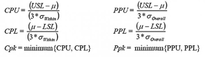
Where:
CPU/CPL = Upper/Lower capability Process Limit
PPU/PPL = Upper/Lower potential process Limit
μ = XBar = (mean of the data)
σWithin = Standard Deviation pooled within subgroups
σOverall = Overall Standard Deviation of the dataset, lot or population
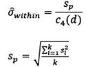
In the equation above, the calculation for the within Standard Deviation of Cpk for equal number subgroups is:
![]()
Where:
Sp = The summation of variance within each
subgroup, i.e. {Σ STDEV2 / k}1/2
k = Number of subgroups
C4 = computes the expected (unbiased) value of the standard deviation of &nindependent normal random variables with (d) degrees of freedom.
η = Total number of samples
d = degrees of freedom
Note: C4 (d) is to be read as: C4 of (d), not C4 times (d). So where do you get the C4 of (d), the unbiased standard deviation value? These come from readily available statistical tables. For example: If (d) = 28 then, C4 is taken at (0.990786)
Also note that the special case of calculating Cpk with a subgroup size of 1.0 can be done with an estimate of standard deviation using the moving range equation (not shown).
The overall standard deviation is much easier to calculate. Here it is taken without respect to subgroups and is given by
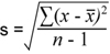
Where:
X = the individual shaft diameter measurements
n = Total Number of data points
XBar = Mean of all (60) data points
See Figure 4.

Let’s take a look now at the potential difference between Cpk & Ppk
In our example, there were 600 shafts made. 10 out of 100 were measured each hour for six hours. 60 data points were accumulated. There are six subgroups of 10 data points. Parts are made on one machine, by one operator, the same way on the same day. We can see that the average standard deviation within subgroups is very close to the overall standard deviation. Therefore, in this particular case, Cpk and Ppk should be very close in value – and they are. (Figure 5)

Note: This example is a two-tailed distribution based on the upper and lower control limits (diameter specification). Therefore, Cpk and Ppk is taken as the lessor value of the two calculations.
Here is where the difference between within and overall standard deviation is apparent. If we pull 30 measurements out of the 60 total that were taken, irrespective of time order, to make 3 unique subgroups, there could be wildly different results (we would never, ever do this). The difference between the lower and upper Ppk values (1.72 vs. 1.37) is +25%. However, the difference for Cpk is (3.13 vs. 1.39) +125%! (Figure 6). The result comes from the data in Figure 3. Cpk calculates the standard deviation of each subgroup and pools the results, whereas Ppk calculates the standard deviation from all data as one continuous matrix.

This example shows the importance of truly understanding the data you are investigating. Ask: How is the data taken? How stable is it? Where is the variation coming from? Is the data trustworthy? How was it organized? Are there enough data points? Will this process generate like results, lot after lot, time after time? Is the statistical confidence level of the capability indices acceptable? As so often is the case, if a decision is going to be made about whether the parts and process are acceptable for production based on a series of initial subgroup “snap-shots,” then it behooves one to really dig into these specifics; so today’s Cpk is not wildly different from the future long-term process capability. Along the way, the most important thing you may discover is how to continuously and confidently verify whether your process is actually in control and truly capable.
References
- Paret M. & Sheehy P. “Being in Control” Quality Canada, Summer 2009.
- Capability Analysis (Normal) Formulas – Capability Statistics, http://www.minitab.com/support/answers/answer.aspx?ID=294
- Paret M. Process Capability Statistics: Cpk vs. Ppk
- Bower, K.M. “Cpk vs. Ppk” ASQ Six Sigma Forum, April 2005, www.asq.org/sixsigma
- Symphony Technologies Pvt Ltd “Measuring Your Process Capability”. www.symphonytech.com
- Cheshire A. “Questions about Capability Statistics – Part 1” September 19, 2011
- Pyzdek, Thomas “The Six Sigma Handbook”, McGraw-Hill, 2003 pp. (467-484)
- Statistical Process Control 2nd Edition “Reference Manual,” DaimlerChrysler / Ford Motor Co. /General Motors Corp. Supplier Quality Task Force, July 2005
“Portions of information contained in this publication/book are printed with permission of Minitab Inc. All such material remains the exclusive property and copyright of Minitab Inc. All rights reserved.”


